Making better cheese with IoT and ML
Optimise the cheese making process utilising low-cost IoT and machine learning solutions.
A small cheese factory wanted to improve its production process, focussing on the quality of its product. The key focus was to improve the temperature monitoring in their cold rooms to keep the product fresh and increase shelf-life.
The previous quality control system involved a person going to each cold room every four hours and manually taking the temperature reading from the digital display. This worked well for monitoring during normal working hours, but not during the evenings and over weekends. And of course, assuming nothing goes wrong within four hours. As the factory is based in a rural location, power interruptions occur regularly, and a backup generator is installed. However, it has happened that the generator fails to start which led to some product losses over weekends.
Phase 1 focussed on improved monitoring, which will be discussed briefly, and phase 2 focussed on implementing machine learning, which will be discussed in detail in this blog post.
Phase 1: Improved monitoring
The first step of the project was to implement an Internet-of-Things (IoT) solution to provide real-time monitoring of their refrigeration systems in the cold rooms. While there are a few commercial IoT solutions available, the costs tend to add up quickly when considering the sensors, infrastructure, and cloud hosting fees, especially for a small factory.
A more cost-effective solution was a custom-built IoT device, utilising an ESP32 microcontroller and some off the shelf sensors. A simple web-based app was created and hosted on a local PC.
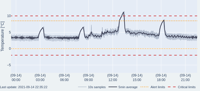
The system measures the temperature inside the cold room, the power consumption of the refrigeration units and the outside ambient temperature. Now, instead of manually taking spot measurements, the real-time temperature is now captured automatically every 30 to 60 seconds which provides more consistent monitoring and more insights into the system operation.
Alarms are sent out if the temperature exceeds the upper or lower limits for 30 minutes, however, there appeared to be alarms consistently every couple of hours which would go back to normal without manual intervention.
Phase 2: Using data for better insights
The implementation of the IoT solution provided improved monitoring and plenty of real-time data that was not available before. The next phase of the project is to implement more advanced analytics, i.e., using the generated data, to gain better insights into the process and system operation.
Three key business needs
1. How can we better implement refrigeration temperature monitoring? We need to understand the regular nuisance alarms and what happens within the control limits.
2. What is the current energy performance of the refrigeration system? Firstly, can we build a good energy model using that data available and can we identify potential energy savings?
3. What needs to be done to implement the changes identified and can is be done cost effectively?
Project approach
- Data preparation: Data ingestion pipeline to be built including data quality processing. This will also allow to add additional data in future.
- Exploratory Data Analysis (EDA): Explore the new data and identify the characteristics and identify potential new features.
- Develop and test ML models: Based on the business needs, develop appropriate models and test performance.
- Summarise outcomes: Discuss findings and next steps for this part of the project.
The data and python notebooks are available on GitHub 🙂
Data preparation
Sensor descriptions and data
A description of the various sensors are located in the sensors_sensor_202107282041.csv. It includes:
- sensor_id to match with the daily data files;
- sensor_type and sensor_uom (unit of measure);
- sensor_ucl and sensor_lcl which are the upper and lower control limits used for alerts; and
- sensor_uucl and sensor_llcl which are the upper upper and lower lower control limits used for alarms.
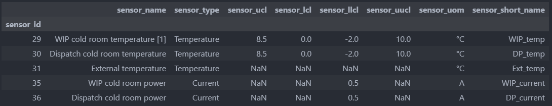
The sensors of interest are the cold room temperatures, cold room power consumption and the external ambient temperature. There are two cold room: the one for work-in-progress (WIP) and one for dispatch (DP).
The IoT system was implemented toward the end of March 2021, which provided around five months’ worth of high-frequency data. Daily data files were received as compressed CSV files, created by the system for backup purposes. The file contains three columns:
- timestamp: the date and time the sensor readings were taken
- value: the raw sensor reading in the unit of measure as per the sensor description file; and
- sensor_id_id: the integer ID of the sensor to match with the sensor description file.
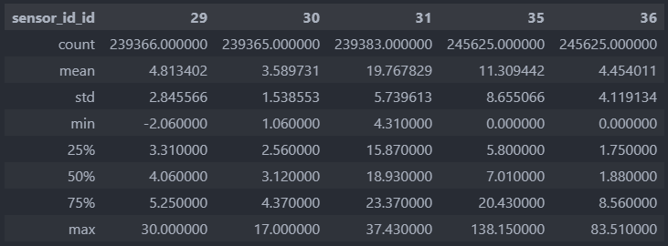
Having a look at the statistics for the raw data, we can see there are about 5000 additional data points for the current readings (32 and 36), which indicates some missing data points. It can also be seen that the temperature readings (29, 30 and 31) have a minimum of -127 which is suspect and will also influence mean and standard deviations depending on how many data point of that value there are.

Data processing
A data pipeline was developed to read the individual compressed CSV data files, combine it in a single data frame and perform some clean up. The following criteria is used to filter bad quality data, as per the real-time monitoring system:
- the value of -99 is assigned to any sensor value which was bad quality or not available;
- the value of -127 indicates bad quality data for some of the temperature sensors; and
- the values of -327 and 327 indicates the bad quality data that is at the extreme limits of the device range.
In this application, temperatures are normally just above zero degrees Celsius and thus values of -99 or -127 are not near normal ranges. There were no data points equal to -99 and no data points at extreme limits, but there were 155 data points equal to -127. After removing these, the statistics look more aligned to the process.
Temperature data was averaged out over five-minute periods to reduce the noise from the raw measurements as the system is slow acting, at least for temperature. The variation in the normal on-off cycle data is slightly reduced but the defrost spike is still prominent.
For the energy analysis, current measurements (a measure of power) were converted to an energy measure, as current changes rapidly and is observed in the noisy current trends. We are also interested in the energy consumption and not the instantaneous values. The voltage at the site is 400V in a three-phase system. An average power factor of 0.85 is assumed. The temperature data for this analysis was averaged out over an hour.
These steps are outlined in data-etl.ipynb.
Exploratory Data Analysis
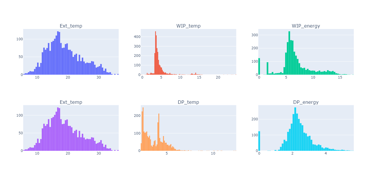
External temperature is normally distributed, which makes sense. The WIP temperature looks as expected with a specific set-point, however, the DP temperature seems to have two different set-points. On energy, we can see periods where the equipment was off (with the peak in the first bin).
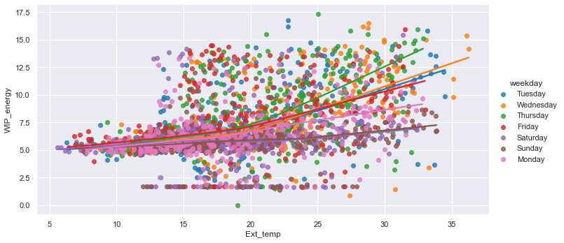
In analysing the timeseries trends (temperature and energy), there appears to be some peaks in energy that match daily temperatures during week days, but not much variation on weekends. The day of the week may be a good feature to include. Energy consumption on Saturdays and Sundays are different from other days during the week as minimal work takes place on weekends. During the week, there is constant movement in and out of the cold room and adding new product.
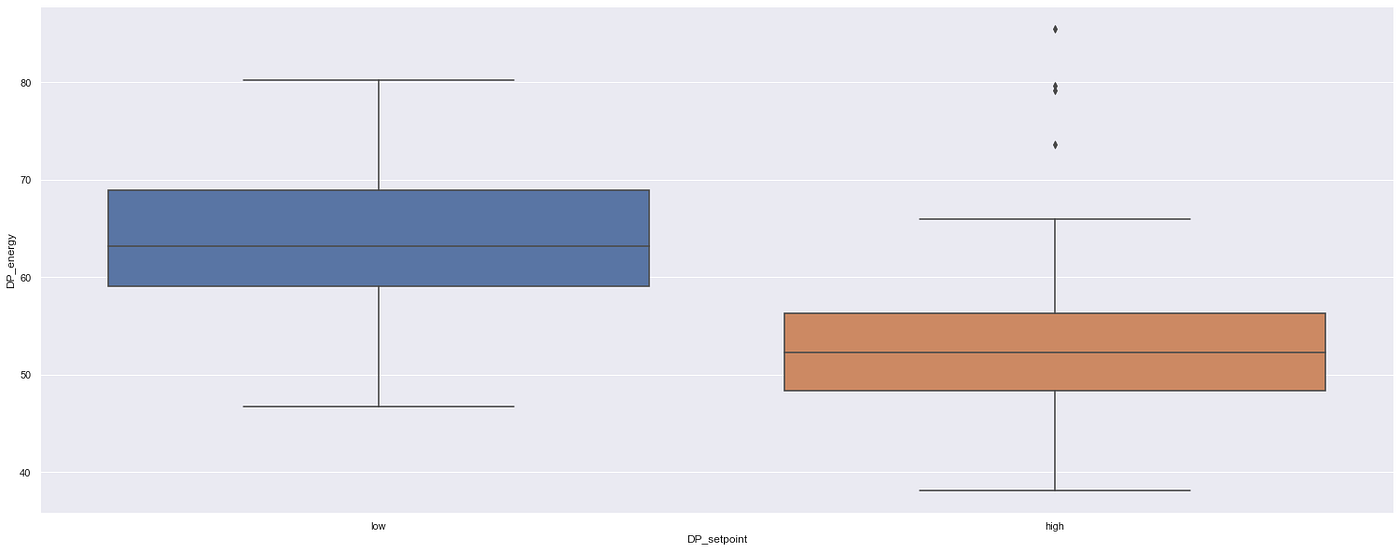
Observing the differences in set-point for the Dispatch cold room, we can split the cold room temperature at 3.5°C to compare the differences in energy consumption for a high set-point (4°C) and a low set-point (2°C). The mean difference is 3 538 kWh/annum, which is about 18%. This implies a potential saving of 18% if it operates at the higher set-point, assuming it does not affect product quality off course. However, we would need to consider the relevant variables over time which can have a significant impact.
These steps are outlined in eda.ipynb.
Using anomaly detection for cold room temperature monitoring
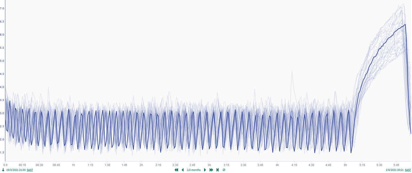
One of the insights in the more consistent monitoring was the prominent automatic defrost cycle that occurs every 6 hours. This was the cause for most of the nuisance alarms. This was not common knowledge and rarely caused concerns with the previous manual readings, except if the readings were taken during this time. The real-time monitoring made this visible, but the nuisance alarms was not aiding adoption of the new system.
One solution to solve the nuisance alarms is to use an autoencoder, a convolutional neural network. There is a well documented example using the Keras library for timeseries anomaly detection using an autoencoder from pavithrasv which was adopted for this analysis. It basically takes the input data and encodes (compress) it, reducing features and then starts to decode the features to reconstruct the original data, while minimising the error. Thus, it is important to ensure the input data is good quality and normal for the process at hand.
We have the temperature trends that follows a six-hourly cycle and is predictable under normal circumstances. After examining the timeseries trends, a good period was identified to use as training data for the autoencoder (between 2021–05–07 16:30 and 2021–05–11 4:20). The difficulty in this approach is working with unlabelled data and visually finding good cycles. A typical cycle was investigated to determine the time steps that were needed to create the training sequences. A typical time step is about 74, which is 6 hours and 15 minutes.
Metrics
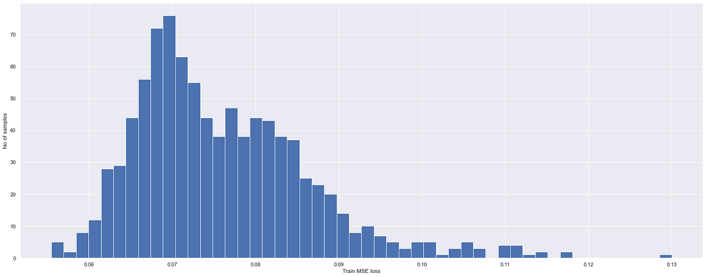
In defining the Keras model, Mean Square Error (MSE) was chosen as the loss function to benefit of penalising larger errors which can be critical for this application. For other parameters the default was used.
Model evaluation and selection
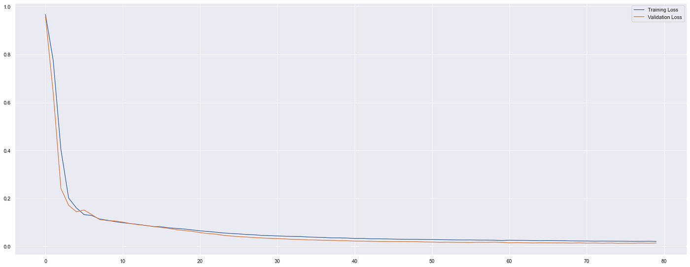
After training, we see the model fits well with both the training and validation data sets. By plotting the MSE, the reconstruction threshold was calculated at the maximum of the training loss at 0.13. Some difficulty was experienced when adjusting parameters too much which led to large losses in the models.
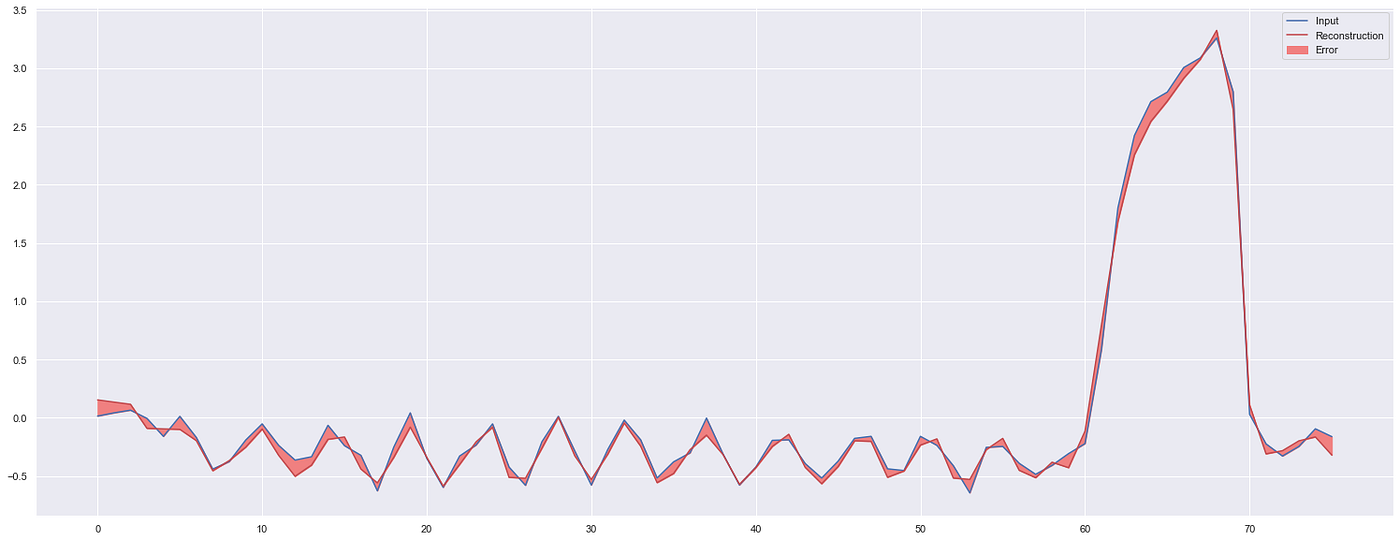
Individual sequences were examined and reconstructed from the model and the error calculated to verify the fit of the model. Using one of the training sequences, we observe a good fit and minimal error. Using some of the detected anomaly sequences, the areas of large errors are clearly seen.

Results
Applying this to all the available data, there as some clear anomalies that we would expect to catch but also some others that may or may not be of importance. Importantly, some set-point shifts were also identified as anomalies which may imply the process is not operating where it should. This is a good first pass using the provided example.
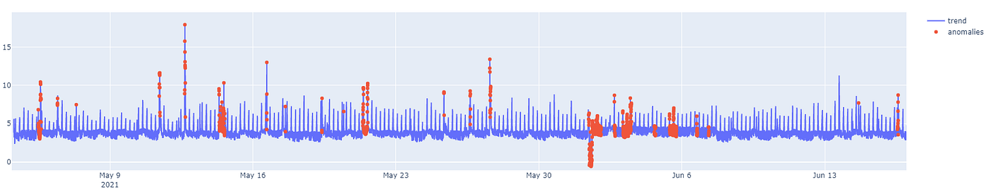
Adjusting the loss function threshold affects to sensitivity of the model to detect anomalies. If the threshold is too high, we may miss periods were the setpoint temperature shift by a degree of two, which may imply using additional energy or reducing product shelf-life.
This is a complex method that can be implemented with some basic knowledge and world class libraries. It can reduce nuisance alarms for our application and should be combined with other methods for a more robust implementation.
These steps are outlined in anomaly-detection-dp.ipynb. A similar analysis was done for the WIP cold room (anomaly-detection-wip.ipynb).
Estimating the energy performance of the refrigeration system
Up until now, the focus has been on the temperature monitoring in the cold room. To build a model to measure energy performance, relevant variables need to be measured. The IoT system measures the outside ambient temperature as well as the current drawn by the refrigeration units. From an energy perspective, the cold room temperature is a set-point rather than a relevant variable. However, this will affect the energy consumption as there appeared to be two distinctive set-points during different periods for the Dispatch cold room.
From a quality perspective, the requirement would be to keep to cold rooms at around 4°C and thus anything colder, implies that more energy would be needed to cool in this particular climate. Thus, our energy model can estimate the difference in energy between the two set-points and estimate potential energy savings.
Defining the model
A simple energy model was developed using regression analysis relating energy consumption to the ambient temperature and set-point temperature. Daily data was used as the data can be noisy in smaller intervals, especially with limited features. The same temperature split was used for the data set as in the EDA phase, i.e. 3.5°C. For the model, the 4°C set-point was used as the baseline and the 2°C set-point as our reporting period, using daily data. The available data points are 53 and 61 for the baseline and reporting periods, respectively, and thus well balanced.
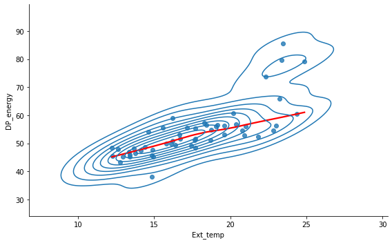
The EDA also showed a correlation between energy consumption and external temperature. We confirm this with the scatter plot for the baseline period and also observe four clear outliers in the top right as well as a slight non-linearity with the lowess line. The outliers were removed from the analysis.
Metrics
Root Mean Square Error (RMSE) was chosen over Mean Absolute Error (MAE) as it penalises large errors. Small deviations from the predicted energy is not that important, but one large value will impact the cumulative energy performance. Another metric is the adjusted R-squared as we have more than one feature, it provides a more robust metric than the R-squared, which increases by adding features. The practical application of this metric is to explain the variability in the energy consumption and give us an indication if we may be missing features.
Model evaluation and selection
The features (external temperature and set-point temperature) were standardised and 25% of the data set was used for testing. As a base reference, a OLS regression model was fitted as the outliers were removed and there was only slight non-linearity. The model yielded a RMSE of 3.83 and an adjusted R-squared of 0.5356 on the test set, which explain about 53% of the variability. This may indicate some missing relevant variables or process control issues.
In order to see if the model can be improved with a more robust algorithm, I opted to use a boosted regression tree, i.e. XGBoost, as it is insensitive to non-normality of features, more easily interpretable and accurate. I included 3 folds for cross validation as it is a small data set using the daily data and a grid search for hyper-parameter tuning. Fairly wide ranges were chosen to find the best parameters, but care was taken in the selected to ensure the model is not complex and potentially overfitted, e.g. max_depth should not go too deep. To make overfitting less likely, I also specified colsample_bytree and subsample parameters so that it uses slightly different data at each step.
The model yielded a RMSE of 3.49 and adjusted R-squared of 0.6147, which is about 8% better than the OLS regression model. The best parameters was at a max_depth of 5 and the sampling parameters were both 0.3, implying an acceptable model that is not overfitted. Having a look at the regression plots for test data, the residuals look randomly distributed with only one point standing out in the Q-Q plot.

Results
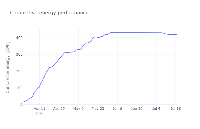
Now we can use the optimised XGBoost model on the reporting period data to predict the energy that would have been consumed at the higher set-point. The cumulative sum of the difference between the predicted and actual energy consumption, will give the additional energy that was consumed during this period. The additional energy consumption was 419 kWh over the period, and adjusting that to represent an annual figure, the predicted additional energy consumption is 2 507 kWh/annum, i.e. about 11% more.
Thus, potentially over a year, the factory would be able to save 2 507 kWh (about 11%) based a more conservative energy model. This is about 70% of mean box plot analysis done in the EDA phase. This is a good saving, especially when running from a diesel generator during power interruptions which adds more cost to the business and carbon emissions.
A few key things to note is that some data was not available, like data regarding production volumes and perhaps how many times the doors were opened and closed (potential additional features). Another is that the energy consumption is affected by ambient temperature, and we are only looking at a few months’ worth of data and therefore is not 100% representative over all seasons.
These steps are outlined in energy-model.ipynb.
Business outcomes and considerations
One of the key findings was the prominent automatic defrost cycle. With this knowledge, the Maintenance Manager wondered why a cold room in another factory, with an identical system, did not have any defrost cycle. As it turns out, that system was not properly commissioned, and it explains why it needed more frequent maintenance and consumed more energy. This has since been corrected, reducing costs for another factory in their organisation.
From the energy analysis, we determined that there is a difference in energy consumption between a set-point of 2°C and 4°C. A reduction of about 11% in energy consumption can make a big difference in the bigger picture, especially considering more self-sustaining energy systems, such as solar energy and batteries. It may have an impact on the capital cost of such a systems as well as the battery capacity.
In contrast, there may be a benefit in lower operating temperature for the cold-room. There may be slightly more energy being consumed, but it may result in a longer shelf-life of the product. This potentially means less food waste and saving energy, when considering the embedded energy in the product already.
Conclusion
This project focussed on extracting value out of a low-cost, custom-build IoT solution with new real-time data. Using simple machine learning techniques for anomaly detection, it can allow personnel to focus on the actual alarms and avoid nuisance alarms. By continuously measuring energy performance, energy and cost savings can be realised.
The application of simple machine learning models implies that a low-cost analytics solution, that is not compute intensive, can be developed that is simple to understand, implement and maintain, while delivering 80% of business value.
Opportunities for improvement
The next step for this phase of the project is to build and integrate the machine learning pipelines into the main IoT solution and providing an interface to retrain and deploy models for testing.
The latter is important not only for model maintenance purposes but also because there was limited data available and there would be a benefit to using a larger and more representative data set.
For anomaly detection, the autoencoder should be combined with the control limits and perhaps statistical process control principles to offer a more robust alarm function.
For the energy model, additional data should also be gathered to add more features and increase the daily data points. The difficulty in this analysis is the limited daily data points that we have available which may imply that the model won’t generalise well in operation.
The notebooks and data is available on GitHub 🙂

0 Comments