While data storage and retrieval are essential first steps, the true value of a data stack lies in its ability to provide real-time analytics and actionable insights. In Part 1, we demonstrated how to replace a traditional process historian with a modern, open-source data stack. In this post, we’ll explore how to add automated data aggregations on the edge to track near real-time energy costs and compare different electricity tariffs to minimise costs.

The analytics gap in traditional systems

The key focus of traditional historians is on data storage and retrieval, typically in the context of an industrial setting and using their built-in tools. Most traditional historians offer some sort of aggregations and calculations, but this is built within their application ecosystem. These often have their own syntax and requires specialised training and skills. Because of this, most users need to interact with the data outside of the historian. Many rely on good old Excel. This may be good for a once off analysis but is generally time consuming and not repeatable (unless you are ingesting these Excel files?!). Some offer integration with BI tools, however querying 10s second data to aggregate data into daily totals is not efficient in these BI tools and can typically overload historians if this is done often. Sometimes these BI tool integrations come with an additional charge as well. All of these increases time to action.

With the increase of data generation and the need to get to actionable insights faster, the traditional historian systems are lagging behind. For more complex reporting and calculations, data is extracted from historians in raw format or in aggregation calculations. Additional business logic is then built externally in other cloud and ETL tools. All of these add latency, cost and complexity, and often needs people with different skillsets. Changing this business logic also becomes quite a task to coordinate between different developers.

Advanced real-time data processing on the Edge

In our previous post, we implemented InfluxDB 3 Core as our edge time-series database. It includes a powerful processing engine for custom Python plugins to process our data, natively as part of the database. The processing engine supports three trigger types: on data write (real-time processing), on schedule (periodic aggregations), or on demand (ad-hoc analysis). This flexibility enables both operational and analytical workloads to coexist on the edge. We can efficiently write data back to the database and use this for visualisation on the edge (or on site).

The advantage is we use processing on the edge with no additional infrastructure needed and data stays with the database, reducing bandwidth requirements and latency. It reduces the need to have scripts running externally, either on-prem or in the cloud, with other tools, reducing complexity and becomes more maintainable. Python skills are also more widely available, and most AI based tools can assist with generating code… Trust but verify!

This capability brings additional challenges to manage as well. The edge infrastructure may need to be scaled up if running intensive workloads, like machine learning, but typically these should just be for inference and not training models. With the vast amount of Python libraries available, there will be security concerns and vulnerabilities to address.

Use case: Time-of-use tariff analysis

Utility energy providers offer different tariff options for different type of consumers, and it means that users may have several options to consider. While flat-rates are simple, Time-of-Use (TOU) tariffs are more complex to evaluate to see which one is more cost effective at the end of the day. With the adoption of renewable energy systems and battery storage, increasing the variability in the grid, many utilities are implementing TOU tariffs or even real-time tariffs to influence consumer behaviour and may be forcing consumers to use more complex tariff structures.

While this can be frustrating for consumers, it also brings opportunities to reduce energy costs by managing the storage systems. Adding the ability to export excess energy to the grid, it allows consumers to not only support the grid during peak times but also reduce their own costs.

In South Africa, Eskom’s TOU tariff includes three periods: Peak (morning and evening rush hours), Standard (business hours), and Off-peak (nights and weekends), with rates varying by season.

Building on top of our home energy dashboard and the data we are collecting, we will be evaluating a fixed cost tariff and a TOU tariff. We want to know what the impact is of changing the tariff and keeping our consumption patterns the same. The consumption pattern is something we can control and change, if needed, in terms of when we discharge the battery and when to utilise the hot water heating boost timers. Having this near real-time view of our energy costs, allows us to take quick action to change consumption where needed.

Implementing the tariff processing plugin

We built a simple Python plugin to aggregate our grid energy consumption data into half-hour increments, converting from power (Watt) to energy (kWh). This is a simple aggregation that runs every half-hour. In addition, we need to classify the TOU periods, Peak, Standard and Off-peak, for every half-hour block. Important to note that there is also a seasonal component with High season being the three winter months and Low being the remaining months of the year, with seasonal adjusted tariffs. There are also subsidies and fixed monthly costs, which have been blended into to rates that we will use.

The plugin was implemented with a single Python .py file, while the latest version allows a module-based folder structure, making code more maintainable. The tariff costs have been hard coded into the Python file for now but will be moved to a proper table or config file. The entry point is process_scheduled_call function. First, we query our grid power tag, grid_power_W for the last 30-minutes and convert it to a pandas data frame. We use normal pandas functions to set the types and resample the data.

Using the resampled timestamps, we use a few helper functions to determine the season and the TOU period, and lookup the TOU tariff rate. We then simply multiply the energy by the specific rate for that half-hour. The fixed tariff is just a simple calculation. Lastly, we use the InfluxDB’s Python SDK to build the InfluxDB line to write to a separate table. We added logging to review execution.

View this gist on GitHub

Using the CLI, we can quickly test the execution of the plugin without writing data to the table. Once happy with the result, we also use the CLI to create the schedule.

Home energy system insights

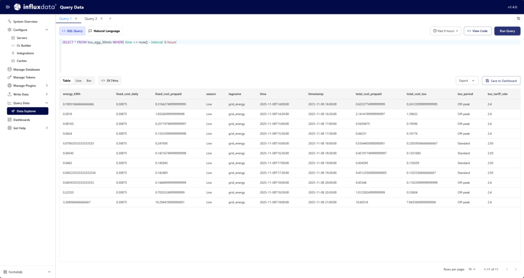
InfluxDB has a web app, Explorer, which allows you to manage your Influx DB instance (Core and Enterprise), including plugins, as well as querying and visualising data. This is valuable to view the execution of the plugins and quickly query the results to verify that they calculate correctly.

Of course, we implemented our dashboards in Grafana, so we added new panels for the tariffs. The first visualisation is a half-hourly comparison between the two tariffs. For each half-hour we can clearly see the cost difference (the first being the TOU tariff and the second lighter bar being the fixed tariff). Note this is only for the energy we consume from the grid and there is no exporting to the grid at the moment. The second visualisation is a cumulative cost trend, showing the impact over the last day.

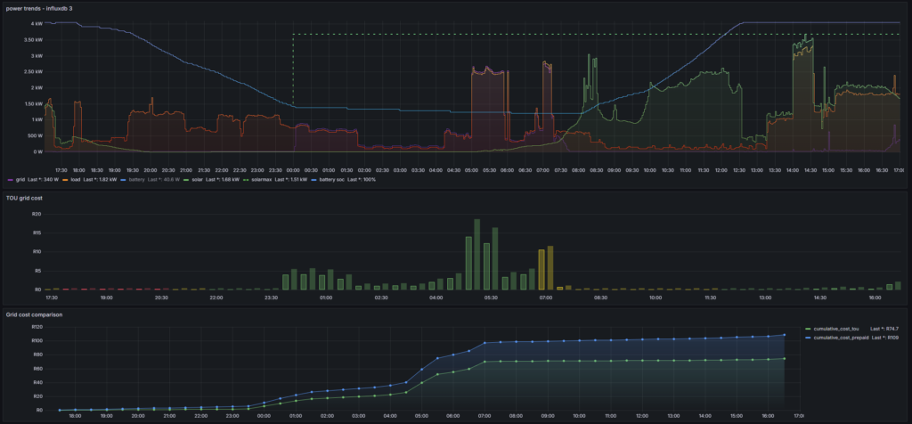
Looking at the power trends panel, we can clearly see the battery discharge starting at 17:00 (shown in the battery power trace), successfully avoiding grid consumption during the peak period (18:00-20:00). The TOU cost panel shows minimal charges during peak times, with most costs occurring during standard and off-peak periods. Over the day shown, the cumulative comparison reveals approximately R34 savings with the prepaid tariff being R109 versus R75 with TOU – a significant difference that validates our optimisation strategy.

The importance of having this near real-time view is still valuable as other loads, such as air conditioning, is not being controlled and can have a significant impact on energy costs. Thus, it enables more proactive energy management that can be addressed in hours, instead of getting a huge bill at the end of the month.

Having the logic of this plugin, we can also apply this directly to our solar energy consumption. This will allow us to calculate the energy, carbon and costs savings we are getting from the solar and battery storage system. We can also estimate (and track if implemented) the benefit of exporting excess solar energy to the grid, using those specific tariffs.

This gives us a near real-time trend on the edge but only for three days, due to using InfluxDB Core. In part one, our data stack uses Azure Data Explorer (ADX) as our long-term cloud storage. Seeing that the plugin is written in Python, we can run the Python script in ADX, with a few tweaks off course, on our historic data. This gives us far better estimate across seasons on a much larger data set. We can also now ingest the new aggregated data directly into ADX for longer term record keeping, reducing the need to run another compute process in the ADX to process the same data. Less costs and more maintainable.

Conclusion

By incorporating automated analytics directly into the data stack, leveraging InfluxDB’s processing engine, we’ve moved beyond simple storage and retrieval to create a system that continuously generates actionable insights, on the edge where it is needed. The same business logic can easily be transferred to the cloud components. The TOU tariff use case demonstrates how automated aggregations can validate optimisation strategies (i.e. changing consumption patterns), enable real-time cost visibility to address issues in hours and not at month end, and provide tracked ROI of renewable energy system payback.

This approach bridges the gap between data collection and actionable insights, reducing latency and complexity while maintaining the simplicity and cost benefits of the modern stack outlined in Part 1. Whether for home energy management or industrial process optimization, building analytics into the data pipeline transforms raw data into continuous, automated intelligence.

As edge computing capabilities continue to evolve, we anticipate moving beyond basic analytics to deploy lightweight machine learning models for predictive insights – bringing AI directly to where decisions are made. The foundation we’ve built with InfluxDB’s processing engine positions us perfectly for this next evolution.